As modellers, our goal should always be to strive towards more realistic abstractions of the real world processes which we simulate. In light of this, it’s not enough to merely increase the accuracy or detail with which we capture behaviour of agents in our simulation models, but we need to ensure the environments within which these agents reside also represent realistic landscapes, depending on the nature of the model which we are building.
Shapefiles store non-topographical geometry, as well as attribute information, pertaining to the spatial features in a data set. In a shapefile, a feature’s geometry is typically stored as a shape comprising of a set of vector coordinates. These days, most geographical maps may be accessed as Geographical Information Systems (GIS) maps directly, however, some applications are still bound to the use of shapefiles (such as the application which inspired this post).
There exists functionality in AnyLogic to deal with both shapefiles and GIS, although, admittedly, I didn’t investigate it too thoroughly before attempting to create my own importation algorithm. In my model, I required each shape to be accessible as a presentation element – discoverable by agents and useable in the execution of functions. Whether or not this is achievable using the latest AnyLogic software – I’m not entirely sure – but here’s a (relatively) simple way to build it yourself.
Firstly, if you’re using shapefiles like I was, you need to extract the data from the .shp and .shx files. The .shp file typically stores spatial information (such as coordinates) whilst the .shx file stores attribute information about the different spatial element shapes (such as actual perimeter, area etc.). Extraction can be easily achieved using a free GIS application, or the shapefiles package in an open-source software like Python (which is what I used). I used the Decimal Degrees (DD) format as an output of the coordinates instead of the common degrees, minutes and seconds format. DD simply returns a decimal x and y value for each coordinate, where positive y coordinates indicate latitudes north of the equator, whilst latitudes south of the equator are represented by negative y values. This is similar for x values, with positive and negative x coordinates representing eastern and western longitudes relative to the Prime Meridian, respectively.
Since AnyLogic links easily to Excel, I recommend you extract your data into two Excel sheets of .xlxs format (one spatial element information file and one attribute information file). Your spatial element file should look something like this:
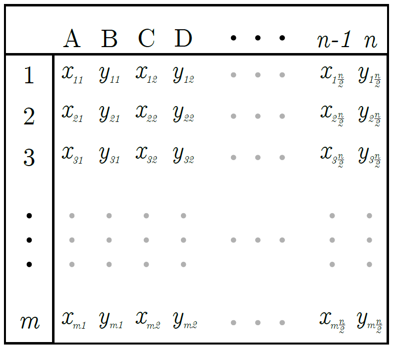
Spatial information of a shape file.
In the shapefile, you have m spatial elements, each being described by n/2 coordinates (The x and y coordinates are stored in the same row – this may be altered according to your preference and the method you used for extraction). Note that the value of n may differ for each element.
Now, what you want is a generic algorithm which will create a polyline for each of the spatial elements in your dataset and fix the vertices of that polyline according to the GIS coordinates stored in the linked Excel spreadsheet. The problem is, in AnyLogic, one typically has to draw presentation elements from the palette before the model is executed. Then, if you know the shape’s name, you may access it during runtime and alter its size, color, or anything else.
But, if we want the algorithm to be generic, then it follows that it should facilitate shapefiles of any number of elements. This means that we need an alternative method of generating presentation shapes as per necessity during runtime. Fortunately, this is achievable using the following snippet of code:
This line of code creates a polyline with the reference name ‘polyline’. Take note – this reference name is only valid for the duration of the function in which the code is called.
So how is this implemented in a simulation?
I recommend making use of a for loop to cycle through your attribute Excel file and deal with each shapes one-by-one. You know, based on the m value in the figure above, how many iterations your for-loop should cycle through. Then, at each line, the number of data points which specify the shape of a particular element may be determined using the built-in AnyLogic function:
where file is the name you gave to the linked Excel attribute file in your model, and rowIndex is the row number (or element) you are currently working on (remember, Excel functions are 1-based, unlike a typical array operation).
Then, at each iteration of the for loop, you can dynamically create a polyline, specify the number of vertices according to the length of the array of coordinate points (or half the length as specified by the Excel operation above, if your x and y coordinates are stored in a single line like mine were) and then incrementally fix each vertex according to the coordinates specified in the Excel file. The code for this operation may look something like this:
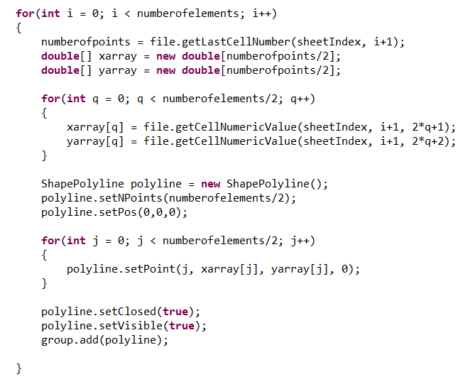
Briefly stepping through the operations in the code snippet:
- Create a for loop which cycles through all of the elements in the linked attribute file (m elements)
- At each element, determine the number of coordinate points which specify its shape. Take note that the designated line with which we are working is represented as i+1 since arrays are zero-based, but the linked Excel sheet is 1-based.
- Create two arrays which store the x and y values extracted from the Excel sheet. This could be one array, but for the sake of simplicity, let’s keep it as two. Take note that these arrays are half the length of the number of points since, in my case, the x and y values were stored together in one line in the Excel file, but now I want to separate them.
- Create a for loop which steps through the line of coordinates and saves the corresponding x and y values into the correct arrays. Note the manner in which the correct row-column combination is selected in this case: the row is determined by the counter of the initial for loop (the one which moves vertically through each of the the spatial elements) whilst the row is specified by manipulating the local counter to only select every second element in the line as either an x or a y coordinate.
- Once the coordinates have been saved, a new polyline must be dynamically created. This is given the local name of ‘polyline’ in this example, but it could be anything.
- Specify the number of vertices this polyline should have (note that this could also be determined as the length of the xarray or yarray established previously).
- Fix the initial position of the polyline so that all distances are relative to the origin.
- Step through each vertex and set it according to the corresponding x- and yarray values which were previously saved.
- Important – set the polyline as ‘closed’ to ensure the final point is automatically joined back to the initial point.
- Make the polyline visible and add it to a group (which should have been created prior to model execution) so that the polyline may be accessible at a later stage for any further modification or other use.
This algorithm should plot in your model, the corresponding elements which were stored in your shapefile. In the case of my application, the shapefile concerned was that of a sugarcane farm. The corresponding shape of the fields existing on that farm, as specified in the shapefile and then extracted and plotted in AnyLogic using the approach described, is shown below:
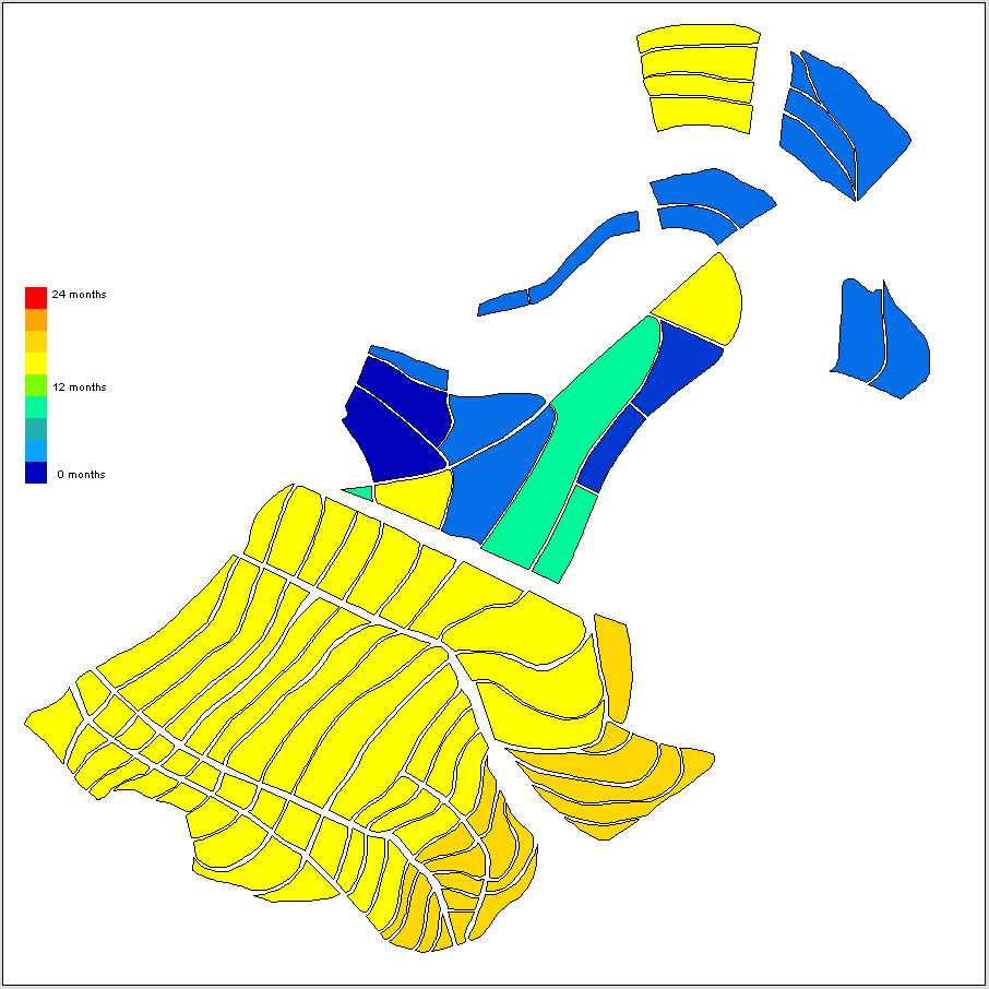
As may be seen, fields have been coloured according to the age of the sugarcane which grows in each field. This information is accessed through the attribute file which was mentioned earlier. I’ll discuss the use of this information in a follow up post.
There are some other complications which must be overcome using this approach:
Firstly, depending on which in the world your shapefile/GIS coordinate information comes from, your data points may be offset from the origin of your simulation space owing to the DD value. For example, South Africa (which is where this shapefile comes from), is located at roughly negative 30 decimal degrees latitude and 31 decimal degrees longitude. This means that, although each vertex in of the imported polylines will be correct relative to the other vertices, the entire shape is going to be offset by a set value within the simulation model and won’t necessarily appear where you want it.
I overcame this error by establishing and x and y offset in my network of shapes. Very simply, I saved the first x and y value in which appear in the shapefile as the offsets and subtracted this value from each other coordinate which I read in. This meant the first point itself is fixed at the origin, and all further points are placed relative to that.
The scale of your data will also determine how it appears when incorporated into your model. This may be overcome by implementing a suitable, fixed scaling factor to each coordinate as it is read into the x- and y arrays. The scale should ideally be dynamically determined, since different shapefiles will require different scales, but this will also be covered in a follow up blog post.
So there you have it, a DIY algorithm which allows you to import your GIS data and recreate the shapes as polylines within your simulation space. This now means your shapes are accessible and may be easily incorporated into your agent’s decision making process and, importantly, benefitting from all of the built in functions which are pertinent to presentation shapes in the AnyLogic library.